NESSUS Hybrid AMV+ - Multimodal Adaptive Importance Sampling

NESSUS Advanced Mean Value with Iterations (AMV+) [1]

NESSUS Advanced Mean Value with Iterations (AMV+) is a most probable point (MPP) based analytical method. It provides a significant improvement over MV, where first it uses approximation to estimate MPP and then performs additional iterations when locating the MPP in order to obtain a more accurate result. A new Taylor series approximation is used for each new MPP and the process is repeated until method converges on an MPP (i.e. no significant change in MPP over a few iterations) or 10 iterations are completed. AMV+ uses finite difference approximations to estimate the gradients. The step size can be set using the Finite Difference Step Size option available but care should be taken for non normal variables that the finite difference step does not move outside of the feasible range of the variable. The method does not support non-smooth responses and failed runs as it is a gradient based method. This method generally requires less than a couple hundred evaluations to compute a probability for less than 10 design variables. AMV+ should always be preferred to MV method. This method should not be used with discrete design variables or discrete response variables. Multiple local MPPs may induce error in the probability estimation by this method and that error tends to be most pronounced for large probabilities of failure.

Advanced Mean Value (AMV) improves the mean value method by using a correction for errors introduced from the truncation of a Taylor's series. The AMV model is defined as:

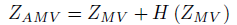
where H(Z_MV) is defined as the difference between the values of Z_MV and Z calculated at the Most Probable Point Locus (MPPL) of Z_MV. The MPPL is defined by connecting all the MPP's for different z values. The MPPL of Z_MV is generally nonlinear curve in the u-space. The key to the AMV method is the reduction of the truncation error by replacing higher-order terms H(X) by a simplified function H(Z_MV) dependent on Z_MV. Ideally H(Z_MV) function should be based on the exact MPPL of the Z-function but AMV simplifies the procedure by using MPPL of Z_MV. Thus optimization of truncation error is not optimum.

Analyzer does not provide AMV but it provides an even better method AMV+. This is an improvement over AMV by using an improved expansion point, which is done by an iteration procedure. Based initially on Z_MV and by keeping track of the MPPL, the exact MPP for a limit state Z = z can be computed to establish the AMV+ model defined as:

where x* is the converged MPP for Z = z. The variables X are generally non-normal and dependent, thus AMV+ model which is linear is in X-space. The above equation provides an initial estimate of the curvature (about the MPP) in the u-space that can be used for approximate probability of failure analysis. The steps followed by AMV+ could be summarized as follows:

Construct mean based response function based on the mean values of the design variables and use it as initial guess for MPP
Use the AMV approximation to come up with a better MPP.
Perform a curve fit operation and then we will have a new MPP
The above steps are performed until the MPP converges or 10 iterations are completed.

Special caution should be used when using probability values in cases where the method has not been able to converge on an MPP. In such cases some experimentation can be carried on to vary the Finite Difference Step Size option.

Multimodal Adaptive Importance Sampling (MAIS)

Multimodal adaptive importance sampling (MAIS) [2,3] is a variation of importance sampling that allows for the use of multiple sampling densities, making it better suited for cases where multiple sections of the limit state are highly probable. MAIS methods require the MPP as a starting point. MAIS efficiency over Monte Carlo increases as the probability of failure decreases. MAIS can be used as an improvement or verification of the probability calculations when using FORM, AMV+. MAIS is performed through the following steps:

1. Generate n initial samples using a sampling density centered at the MPP.

2. Find k “representative points” from these samples:

a. Select the sample with the largest true probability of occurrence.

b. Eliminate all samples within a specified distance (e.g., ) of this point.

c. Repeat steps a. and b. until all samples are exhausted.

3. Calculate the coefficient of variation COV from the n samples:

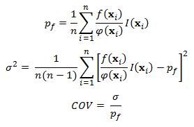
where is the multimodal sampling density function defined below (initially, it is the sampling density function centered at the MPP).

4. Use the k representative points to construct a multimodal sampling density .

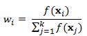
a. Calculate the weight for each representative point, which is based on its probability density relative to that of the other representative points:

b. The multimodal sampling density is then the weighted sum of the probability densities centered at the representative points:

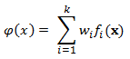
where is the true probability density with the mean shifted to the representative point.

5. Generate n samples using .

6. Repeat steps 2-5 until COV converges. In CENTAUR, we use a convergence tolerance of 0.1 for this step.

7. Generate n samples using the sampling density from the final set of representative points.

8. Calculate p_f and COV from these samples.

9. Repeat Steps 7-8 until COV converges.

Control Parameters

Name	Default Value	Description
Samples	50	This option sets the number of samples to be used in each iteration in the importance sampling.
MaxSamples	1000	This option sets the maximum number of samples in the importance sampling. This does not include the number of evaluations needed to locate the MPP.
Convergence Tolerance	0.05	Coefficient of Variation is used as a convergence tolerance. Coefficient of variation is the ratio of standard deviation of probability of failure to that of probability of failure (in this case estimated probability of failure). The smaller the value of coefficient of variation, more accurate is the estimate of probability. This option can take value between 0 and 1 and is advisable to have a value between 0.01 and 0.2.
Finite Difference Step Size	0.01	This option is used to calculate finite difference step size. The step sizes are determined based on the value of this option multiplied by the mean value of the design variable. Thus if the mean value of the design variable was 5 and the finite difference step size option had the value of 0.1, the actual step size would be 0.1*5 = 0.5. The step size is used by the underlying optimizer trying to locate the MPP. The option expects a value typically within 0 and 1.
Seed	N/A	The seed sets the starting point for the random number generator used with importance sampling. If running multiple tests, keep this value the same if all else is constant. If left blank, Analyzer will generate its own.

References:

1. NESSUS Theoretical Manual, February 17, 2012, Section 8.2-8.3

2. Dey, A. and Mahadevan, S., Ductile Structural System Reliability Analysis Using Adaptive Importance Sampling, Structural Safety, Vol. 20, 1998, pp. 137-154.

3. Zou, T., Mourelatos, Z., Mahadevan, S., and Tu, J., Reliability Analysis of Automotive Body-Door Subsystem, Reliability Engineering and System Safety, Vol. 78, 2002, pp. 315-324.